Generic source#
Description#
The most commonly used type of source is called ‘’GenericSource’’. It can be used to describe a large range of simple source types. With ‘GenericSource’, user must describe 1) particle type, 2) position, 3) direction and 4) energy, see the following example:
from scipy.spatial.transform import Rotation  # used to describe a rotation matrix

MeV = gate.g4_units('MeV')
Bq = gate.g4_units('Bq')
source = sim.add_source('GenericSource', 'mysource')
source.attached_to = 'my_volume'
source.particle = 'proton'
source.activity = 10000 * Bq
source.position.type = 'box'
source.position.size = [4 * cm, 4 * cm, 4 * cm]
source.position.translation = [-3 * cm, -3 * cm, -3 * cm]
source.position.rotation = Rotation.from_euler('x', 45, degrees=True).as_matrix()
source.direction.type = 'iso'
source.energy.type = 'gauss'
source.energy.mono = 80 * MeV
source.energy.sigma_gauss = 1 * MeV
All parameters are stored into a dict-like structure (a Box). Particle
can be ‘gamma’, ‘e+’, ‘e-’, ‘proton’ (all Geant4 names). The number of
particles that will be generated by the source can be described by an
activity source.activity = 10 * MBq or by a number of particle
source.n = 100.
The positions from where the particles will be generated are defined by a shape (‘box’, ‘sphere’, ‘point’, ‘disc’), defined by several parameters (‘size’, ‘radius’) and orientation (‘rotation’, ‘center’). The direction are defined with ‘iso’, ‘momentum’, ‘focused’ and ‘histogram’. The energy can be defined by a single value (‘mono’) or Gaussian (‘gauss’).
Available shapes are: “sphere”, “point”, “box”, “disc” and “cylinder”.
Particle type#
The particle type can be set to any valid Geant4 name
(e.g. "gamma", "e+", "e-"”, "proton"):
source.particle = "gamma"
It is also possible to use ions with the key word “ion” followed by Z and A.
Source of ion can be set with the following (see test013):
source1 = sim.add_source('GenericSource, 'ion1')
source1.particle = 'ion 9 18'  # Fluorine18
source2 = sim.add_source('GenericSource, 'ion2')
source2.particle = 'ion 53 124'  # Iodine 124
Source of ion can be set with the following (see test013)
source1 = sim.add_source('GenericSource, 'ion1')
source1.particle = 'ion 9 18'  # Fluorine18
source2 = sim.add_source('GenericSource, 'ion2')
source2.particle = 'ion 53 124'  # Iodine 124
Note that the ion will only be simulated if the decay is enabled.
sim.physics_manager.enable_decay = True
GATE also provide a back_to_back particle, which is an alias for colinear
gamma pairs of 511 keV.
source.particle = "back_to_back"
Particle initial position#
The positions from were the particles will be generated are defined by a shape
(e.g. “point”, “box”, “sphere”, “disc”, “cylinder”), defined by several parameters (“size”, “radius”)
and orientation (“rotation”, “center”).
A translation relative to the attached_to volume can also be set.
Here are some examples (mostly from test010_generic_source.py):
source.position.type = "point"
source.position.translation = [0 * cm, 0 * cm, -30 * cm]
source.position.type = "sphere"
source.position.radius = 5 * mm
source.position.translation = [-3 * cm, 30 * cm, -3 * cm]
source.position.type = "disc"
source.position.radius = 5 * mm
source.position.translation = [6 * cm, 5 * cm, -30 * cm]
source.position.type = "box"
source.position.size = [4 * cm, 4 * cm, 4 * cm]
source.position.translation = [8 * cm, 8 * cm, 30 * cm]
source.position.type = "cylinder"
source.position.radius = 5 * mm
source.position.dz = 300 * mm / 2.0
source.position.translation = [8 * cm, 8 * cm, 30 * cm]
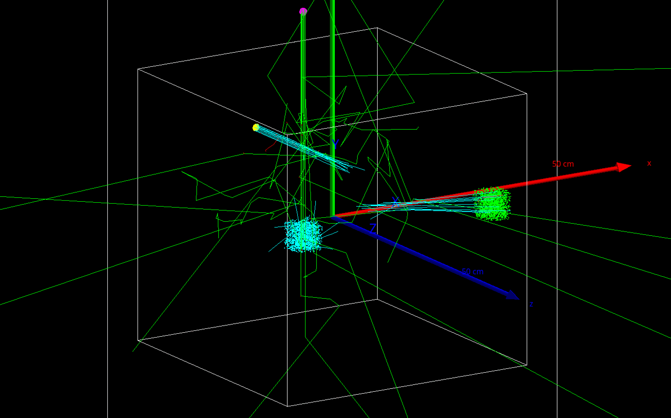
Source position visualization#
A GenericSource can draw a point cloud sampled from its position
distribution in the Geant4 visualization scene. This is useful to check
the source shape, translation, rotation, or attachment before running a
large simulation.
The same method is also available for source classes that inherit from
GenericSource. See source definitions here for
source inheritance details.
The following figure is generated from test file test010_generic_source_visu.py.
It shows the position distribution of 5 different sources with different color:
Enable simulation visualization and set the source visualization parameters
before sim.run():
sim.visu = True
sim.visu_type = "qt"

source = sim.add_source("GenericSource", "mysource")
source.position.type = "sphere"
source.position.radius = 5 * cm
source.visualization.count = 2000
source.visualization.color = "red"
source.visualization.size = 3
The visualization of the source is only available with "qt".
The count parameter controls the number of sampled positions. Values
larger than 10000 are reduced to 2000. The size parameter controls the
screen size of the markers and must be in the range (0, 20); otherwise
the default value 3 is used.
The color parameter can be one of "white", "grey", "gray",
"black", "brown", "red", "green", "blue", "cyan",
"magenta", or "yellow". It can also be an RGB or RGBA list with
components between 0 and 1:
source.visualization.color = [0.0, 0.5, 1.0, 0.7]
This point cloud only represents the source initial position distribution at initialization time. If the source is attached to a volume that moves during the run, this visualization does not show the updated source distribution after the volume movement.
Particle initial direction#
direction.type = 'iso'assigns directions to primary particles based on 𝜃 and 𝜙 angles in a spherical coordinate system. By default, 𝜃 varies from 0° to 180° and 𝜙 varies from 0° to 360° (such that any direction is possible). You can define the 𝜃 and 𝜙 ranges with minimum and maximum values as follows:source.direction.type = "iso" source.direction.theta = [0, 10 * deg] source.direction.phi = [0, 90 * deg]
Geant4 defines the direction as: - x = -sin𝜃 cos𝜙; - y = -sin𝜃 sin𝜙; - z = -cos𝜃.
So 𝜃 is the angle in XOZ plane, from -Z to -X; and 𝜙 is the angle in XOY plane from -X to -Y.

direction.type = 'momentum'specifies a fixed direction for the primary particles using a momentum vector [x, y, z].source.direction.type = "momentum" source.direction.momentum = [0,0,1]
direction.type = 'focused'configures the primary particles to be emitted such that they converge towards a specified focus point. The focus point is set using a coordinate array [x, y, z] that defines its position.source.position.type = "disc" source.position.radius = 2 * cm source.direction.type = "focused" source.direction.focus_point = [1 * cm, 2 * cm, 3 * cm]
direction.type = 'histogram', same as'iso', but allows you to emit primary particles with directional distributions weighted by custom-defined histograms for 𝜃 (theta) and 𝜙 (phi) angles.source.direction.type = "histogram" source.direction.histogram_theta_weights = [1] source.direction.histogram_theta_angles = [80 * deg, 100 * deg] source.direction.histogram_phi_weights = [0.3, 0.5, 1, 0.5, 0.3] source.direction.histogram_phi_angles = [60 * deg, 70 * deg, 80 * deg, 100 * deg, 110 * deg, 120 * deg]
See figure below, left:
# Example A
source.direction.type = "histogram"
source.direction.histogram_phi_angles = [70 * deg, 110 * deg]
source.direction.histogram_phi_weights = [1]
See figure below, right:
# Example B
source.direction.type = "histogram"
source.direction.histogram_phi_angles = [70 * deg, 80 * deg, 90 * deg, 100 * deg, 110 * deg]
source.direction.histogram_phi_weights = [1, 0, 1, 0]


Using source.direction_relative_to_attached_volume = True will make
your source direction change following the rotation of that volume.
Polarization#
polarization = '[1, 0, 0]' assigns a polarization to primary particles (gamma).
The polarization is defined in the particle coordinate system with the
Stokes parameters [Q, U, V].
Do not forget to use an adequate physics list. You can define the polarization as follows:
source.polarization = [1, 0, 0] # linear polarization (horizontal)
source.polarization = [-1, 0, 0] # linear polarization (vertical)
source.polarization = [0, 1, 0] # linear polarization (45°)
source.polarization = [0, -1, 0] # linear polarization (-45°)
source.polarization = [0, 0, 1] # circular polarization (right)
source.polarization = [0, 0, -1] # circular polarization (left)
source.polarization = [0, 0, 0] # unpolarized
sim.physics_manager.physics_list_name = "G4EmLivermorePolarizedPhysics"
Acceptance Angle#
It is possible to configure an angular_acceptance on the direction of a source. This mechanism controls which particles are accepted based on their direction relative to one or more target_volumes. Two checks can be enabled independently and combined:
enable_intersection_check: accepts the particle only if its trajectory intersects the target volume(s). This is useful for SPECT imaging to limit particle creation to those that have a chance of reaching the detector.enable_angle_check: accepts the particle only if its direction lies within a given angular tolerance relative to a reference vector.
The behavior when a particle fails a check is controlled by policy:
"Rejection"withskip_policy="ZeroEnergy": the particle is kept but its energy is set to 0 (not tracked). This preserves consistency with the required activity and timestamps — no solid angle scaling is needed."Rejection"withskip_policy="SkipEvents": the event is discarded and retried. Slightly faster but the total number of events becomes unpredictable."ForceDirection": the particle direction is forced toward the target volume.
Example using intersection check with rejection (ZeroEnergy):
source = sim.add_source("GenericSource", "mysource")
source.direction.angular_acceptance.policy = "Rejection"
source.direction.angular_acceptance.skip_policy = "ZeroEnergy"
source.direction.angular_acceptance.target_volumes = ["spect_detector"]
source.direction.angular_acceptance.enable_intersection_check = True
Example combining intersection and angle checks:
source = sim.add_source("GenericSource", "mysource")
source.direction.angular_acceptance.policy = "Rejection"
source.direction.angular_acceptance.skip_policy = "SkipEvents"
source.direction.angular_acceptance.target_volumes = ["spect_detector"]
source.direction.angular_acceptance.enable_intersection_check = True
source.direction.angular_acceptance.enable_angle_check = True
source.direction.angular_acceptance.angle_check_reference_vector = [0, 0, -1]
source.direction.angular_acceptance.angle_tolerance_max = 20 * sim.unit.deg
See for example test028 test files for more details (in particular test028_ge_nm670_spect_4_acc_angle_helpers.py).
For details on how Geant4 defines particle directions using 𝜃 and 𝜙 angles, see the Particle initial direction section.
Note
Historical note:
Until March 2022, this feature was called
angle_acceptance_volumewith a different structure.From March 2022 to November 2025, it was called
acceptance_angle(i.e.source.direction.acceptance_angle), with propertiesvolumes,intersection_flag,normal_flag,normal_vector, andnormal_tolerance.From November 2025 onwards, it was renamed to
angular_acceptanceand the properties were refactored:acceptance_angleproperty (pre Nov 2025)angular_acceptanceproperty (current)volumestarget_volumesintersection_flagenable_intersection_checknormal_flagenable_angle_checknormal_vectorangle_check_reference_vectornormal_toleranceangle_tolerance_max(implicit)
policy("Rejection"or"ForceDirection")
Half-life#
You can instruct GATE to decrease the activity according to an exponential
decay by setting the parameter half_life. Example:
source = sim.add_source('GenericSource, 'mysource')
source.half_life = 60 * gate.g4_units.s
Note1: If you set a run_timing_intervals starting at t > 0, the activity set in the source is the activity at t=0.
Note2: If you do not set the half_life for an ion, G4 will use it’s own value. Moreover, if you set a run_timing_intervals, by default you the source will decrease without taking into account the run_timing_intervals. To restrict the decay to the run_timing_intervals, you can set the parameter:
sim.run_timing_intervals = [[18 * sec, 28 * sec]]
source.user_particle_life_time = 0
Time Activity Curves (TAC)#
Alternatively, user can provide a TAC (Time Activity Curve) by means of two vectors (times and activities):
starting_activity = 1000 * Bq
half_life = 2 * sec
times = np.linspace(0, 10, num=500, endpoint=True) * sec
decay = np.log(2) / half_life
activities = [starting_activity * np.exp(-decay * t) for t in times]
source.tac_times = times
source.tac_activities = activities
During the simulation, the activity of this source will be updated
according to the current simulation time with a linear interpolation of
this TAC. If the simulation time is before the first time or above the
last one in the times vector, the activity is considered as zero.
The number of elements in the times linspace (here 500) defined the
accuracy of the TAC. See example test052.
Energy#
Mono#
energy.type = "mono" corresponds to a single energy value to be used
for every particle.
source.energy.type = "mono"
source.energy.mono = 1 * MeV
Range#
energy.type = "range" corresponds to a range of energy values between
min_energy and max_energy with a uniform random distribution.
source.energy.type = "range"
source.energy.min_energy = 3 * keV
source.energy.max_energy = 57 * keV
Gauss#
energy.type = "gauss" allows to produce particles according to a
normal distribution with:
μ =
source.energy.monoσ =
source.energy.sigma_gauss
source.energy.type = "gauss"
source.energy.mono = 140 * MeV
source.energy.sigma_gauss = 10 * MeV
Spectra#
Discrete energy spectrum
One can configure a generic source to produce particles with energies depending on weights. To do so, one must provide two lists of the same size: one for energies, one for weights. Each energy is associated to the corresponding weight. Probabilities are derived from weights simply by normalizing the weights list.
1252 isotopes spectra are provided through the get_spectrum function:
spectrum = gate.sources.utility.get_spectrum("Lu177", spectrum_type, database="icrp107")
where spectrum_type is one of “gamma”, “beta-”, “beta+”, “alpha”, “X”, “neutron”,
“auger”, “IE”, “alpha recoil”, “annihilation”, “fission”, “betaD”, “b-spectra”. From this list,
only b-spectra is histogram based (see next section), the rest are discrete. database can be “icrp107” or “radar”.
ICRP107 data comes from [ICRP, 2008. Nuclear Decay Data for Dosimetric Calculations. ICRP Publication 107. Ann. ICRP 38] with the data from the [Supplemental material]. [Direct link to the zipped data]
The source can be configured like this:
source = sim.add_source("GenericSource", "source")
source.particle = "gamma"
source.energy.type = "spectrum_discrete"
source.energy.spectrum_energies = spectrum.energies
source.energy.spectrum_weights = spectrum.weights
For example, using this:
source.energy.spectrum_energies = [0.2, 0.4, 0.6, 0.8, 1.0, 1.2, 1.4, 1.6, 1.8]
source.energy.spectrum_weights = [0.2, 0.4, 0.6, 0.8, 1.0, 0.8, 0.6, 0.4, 0.2]
The produced particles will follow this pattern:

Histogram for beta spectrum
One can configure a generic source to produce particles with energies according to a given histogram. Histograms are defined in the same way as numpy, using bin edges and histogram values.
Several spectra are provided through the get_spectrum function. You can use icrp107 data, or radar data. Radar data comes from [doseinfo-radar] ([direct link to the excel file]).
spectrum = gate.sources.utility.get_spectrum("Lu177", "beta-", database="radar")
The source can be configured like this:
source = sim.add_source("GenericSource", "source")
source.particle = "e-"
source.energy.type = "spectrum_histogram"
source.energy.spectrum_energy_bin_edges = spectrum.energy_bin_edges
source.energy.spectrum_weights = spectrum.weights
For example, using this (which is what you get from get_spectrum(“Lu177”, “beta-”, database=”radar”)):
source.energy.spectrum_energy_bin_edges = [
 0.0, 0.0249, 0.0497, 0.0746, 0.0994, 0.1243, 0.1491,
 0.174, 0.1988, 0.2237, 0.2485, 0.2734, 0.2983, 0.3231,
 0.348, 0.3728, 0.3977, 0.4225, 0.4474, 0.4722, 0.497,
]
source.energy.spectrum_weights = [
 0.135, 0.122, 0.109, 0.0968, 0.0851, 0.0745, 0.0657,
 0.0588, 0.0522, 0.0456, 0.0389, 0.0324, 0.0261, 0.0203,
 0.015, 0.0105, 0.00664, 0.00346, 0.00148, 0.000297,
]
The produced particles will follow this pattern:

Interpolation
Not yet available in GATE.
Predefined energy spectrum for beta+#
There is some predefined energy spectrum of positron (e+):
source = sim.add_source('GenericSource, 'Default')
source.particle = 'e+'
source.energy.type = 'F18'  # F18 or Ga68 or C11 ...
It means the positrons will be generated following the (approximated)
energy spectrum of the F18 ion. Source code is
GateSPSEneDistribution.cpp. Energy spectrum for beta+ emitters are
available : F18, Ga68, Zr89, Na22, C11, N13, O15, Rb82. See
http://www.lnhb.fr/nuclear-data/module-lara. One example is available in
test031.
Confined source#
There is a confine option that allows to generate particles only if
their starting position is within a given volume. See
phantom_nema_iec_body in the contrib folder. Note that the source
volume MUST be larger than the volume it is confined in. Also, note that
no particle source will be generated in the daughters of the confine
volume.
All options have a default values and can be printed with
print(source).
This example confines a Xe133 source within a Trd volume (see Details: Volumes) named “leftLung”:
myConfSource = sim.add_source("GenericSource", "myConfSource")
myConfSource.attached_to = "leftLung"
myConfSource.particle = "ion 54 133"
myConfSource.position.type = "box"
myConfSource.position.size = sim.volume_manager.volumes[myConfSource.attached_to].bounding_box_size
myConfSource.position.confine = "leftLung"
myConfSource.direction.type = "iso"
myConfSource.activity = 1000 * Bq
Reference#
- class GenericSource(*args, **kwargs)[source]#
GenericSource close to the G4 SPS, but a bit simpler. The G4 source created by this class is GateGenericSource.
User input parameters and default values:
activity:
Default value: 0
Description: Activity of the source in Bq (exclusive with ‘n’)
attached_to:
Default value: world
Description: Name of the volume to which the source is attached.
direction:
Default value: {‘type’: ‘iso’, ‘theta’: [0, 3.141592653589793], ‘phi’: [0, 6.283185307179586], ‘momentum’: [0, 0, 1], ‘focus_point’: [0, 0, 0], ‘sigma’: [0, 0], ‘angular_acceptance’: {‘policy’: None, ‘skip_policy’: ‘SkipEvents’, ‘max_rejection’: 10000, ‘target_volumes’: [], ‘enable_intersection_check’: False, ‘enable_angle_check’: False, ‘angle_check_reference_vector’: [0, 0, 1], ‘angle_check_proximity_distance’: 0.0, ‘angle_tolerance_proximal’: 1.5707963267948966, ‘angle_tolerance_min’: 0.0, ‘angle_tolerance_max’: 0.10471975511965978}, ‘accolinearity_flag’: False, ‘accolinearity_fwhm’: 0.008726646259971648, ‘histogram_theta_weights’: [], ‘histogram_theta_angles’: [], ‘histogram_phi_weights’: [], ‘histogram_phi_angles’: []}
Description: Define the direction of the primary particles
direction_relative_to_attached_volume:
Default value: False
Description: Should we update the direction of the particle when the volume is moved (with dynamic parametrisation)?
dynamic_params (set internally, i.e. read-only):
Default value: None
Description: Dictionary of dictionaries, where each dictionary specifies how the parameters of this object should evolve over time during the simulation. You cannot set this parameter directly. Instead, use the ‘add_dynamic_parametrisation()’ method of your object.If None, the object is static (default).
end_time:
Default value: None
Description: End time of the source
energy:
Default value: {‘type’: ‘mono’, ‘mono’: 0, ‘sigma_gauss’: 0, ‘is_cdf’: False, ‘min_energy’: None, ‘max_energy’: None, ‘spectrum_type’: None, ‘spectrum_weights’: [], ‘spectrum_energies’: [], ‘histogram_weight’: [], ‘histogram_energy’: [], ‘spectrum_energy_bin_edges’: [], ‘spectrum_histogram_interpolation’: None}
Description: Define the energy of the primary particles
half_life:
Default value: -1
Description: Half-life decay (-1 if no decay). Only when used with ‘activity’
ion:
Default value: {‘Z’: 0, ‘A’: 0, ‘E’: 0}
Description: If the particle is an ion, you must set Z: Atomic Number, A: Atomic Mass (nn + np +nlambda), E: Excitation energy (i.e. for metastable)
mother:
Deprecated: The user input parameter ‘mother’ is deprecated. Use ‘attached_to’ instead.
n:
Default value: 0
Description: Number of particle to generate (exclusive with ‘activity’)
name (must be provided):
Default value: None
particle:
Default value: gamma
Description: Name of the particle generated by the source (gamma, e+ … or an ion such as ‘ion 9 18’)
polarization:
Default value: []
Description: Polarization of the particle (3 Stokes parameters).
position:
Default value: {‘type’: ‘point’, ‘radius’: 0, ‘sigma_x’: 0, ‘sigma_y’: 0, ‘size’: [0, 0, 0], ‘translation’: [0, 0, 0], ‘rotation’: array([[1., 0., 0.],, [0., 1., 0.],, [0., 0., 1.]]), ‘confine’: None, ‘dz’: None}
Description: Define the position of the primary particles
start_time:
Default value: None
Description: Starting time of the source
tac_activities:
Default value: None
Description: TAC: Time Activity Curve, this set the vector for the activities. Must be used with tac_times.
tac_times:
Default value: None
Description: TAC: Time Activity Curve, this set the vector for the times. Must be used with tac_activities.
user_particle_life_time:
Default value: -1
Description: FIXME
visualization:
Default value: {‘count’: 2000, ‘color’: ‘yellow’, ‘size’: 2}
Description: count is the number of particles to visualize, color is the color of the visualized particles and size is their size (in mm).
weight:
Default value: -1
Description: Particle initial weight (for variance reduction technique)
weight_sigma:
Default value: -1
Description: if not negative, the weights of the particle are a Gaussian distribution with this sigma
Confine Source to Detector Volumes#
OpenGATE allows for the simulation of intrinsic radioactivity within detector materials, such as the natural background radiation arising from Lutetium-176 in LSO/LYSO crystals.
This functionality is achieved by defining a radioactive source and explicitly confining its spatial distribution to specific volumes within the detector geometry (e.g., the Crystal volume). Rather than defining a point source, the simulation generates events stochastically throughout the specified physical volume.
Note
This strategy relies on defining the final layer of the geometry hierarchy as a single, non-repeated volume. This specific volume is then used as the target for source confinement, allowing the simulation to automatically generate the source within every repeated instance of the detector element throughout the entire scanner.
Reference Implementation#
For a comprehensive demonstration of how to define a hierarchical PET scanner geometry and confine the source to crystal volumes, please refer to the following test script:
tests/src/source/testXXX_source_confine_in_the_detector_volume.py