1. User guide
1.1. Introduction & installation
1.1.1. Why this new project ?
The GATE project is more than 15 years old. During this time, it evolves a lot, it now allows to perform a wide range of medical physics simulations such as various imaging systems (PET, SPECT, Compton Cameras, X-ray, etc) and dosimetry studies (external and internal radiotherapy, hadrontherapy, etc). This project led to hundreds of scientific publications, contributing to help researchers and industry.
GATE fully relies on Geant4 for the Monte Carlo engine and provides 1) easy access to Geant4 functionalities, 2) additional features (e.g. variance reduction techniques) and 3) collaborative development to shared source code, avoiding reinventing the wheel. The user interface is done via so-called macro files (.mac) that contain Geant4 style macro commands that are convenient compared to direct Geant4 C++ coding. Note that other projects such as Gamos or Topas rely on similar principles.
Since the beginning of GATE, a lot of changes have happened in both fields of computer science and medical physics, with, among others, the rise of machine learning and Python language, in particular for data analysis. Also, the Geant4 project is still very active and is guaranteed to be maintained at least for the ten next years (as of 2020).
Despite its usefulness and its still very unique features (collaborative, open source, dedicated to medical physics), we think that the GATE software in itself, from a computer science programming point of view, is showing its age. More precisely, the source code has been developed during 15 years by literally hundreds of different developers. The current GitHub repository indicates around 70 unique contributors, but it has been set up only around 2012 and a lot of early contributors are not mentioned in this list. This diversity is the source of a lot of innovation and experiments (and fun!), but also leads to maintenance issues. Some parts of the code are “abandoned”, some others are somehow duplicated. Also, the C++ language evolves tremendously during the last 15 years, with very efficient and convenient concepts such as smart pointers, lambda functions, ‘auto’ keyword … that make it more robust and easier to write and maintain.
Keeping in mind the core pillars of the initial principles (community-based, open-source, medical physics oriented), we decide to start a project to propose a brand new way to perform Monte Carlo simulations in medical physics. Please, remember this is an experimental (crazy ?) attempt, and we are well aware of the very long and large effort it requires to complete it. At time of writing, it is not known if it can be achieved, so we encourage users to continue using the current GATE version for their work. Audacious users may nevertheless try this new system and make feedback. Mad ones can even contribute …
Never stop exploring !
1.1.2. Goals and features
The purpose of this software is to facilitate the creation of Geant4-based Monte Carlo simulations for medical physics using Python as the primary scripting language. The user interface has been redesigned to allow for direct creation of simulations in Python, rather than using macro files.
Some key features of this software include:
Use of Python as the primary scripting language for creating simulations
Multithreading support for efficient simulation execution
Native integration with ITK for image management
Compatibility with Linux, Mac, and potentially Windows operating systems
Convenient installation via a single pip install opengate command
…
1.1.3. Installation (for users, not developers)
You only have to install the Python module with:
pip install opengate
Then, you can create a simulation using the opengate module (see below). For developers, please look the developer guide for the developer installation.
{tip} We highly recommend creating a specific python environment to 1) be sure all dependencies are handled properly and 2) don't mix with your other Python modules. For example, you can use `conda`. Once the environment is created, you need to activate it:
conda create --name opengate_env python=3.10
conda activate opengate_env
pip install opengate
{warning} **WARNING** This does **not** work yet on mac osx with M1 chip (we are working on it). For M1 users, you need to install gate like a developer, see : [developer guide](developer_guide).
Once installed, we recommend to check the installation by running the tests:
opengate_tests
WARNING 1 The first time a simulation is executed, the Geant4 data must be downloaded and installed. This step is automated but can take some times according to your bandwidth. Note that this is only done once. Running opengate_info will print some details and the path of the data.
WARNING 2 With some linux systems (not all), you may encounter an error similar to “cannot allocate memory in static TLS block”. In that case, you must add a specific path to the linker as follows:
export LD_PRELOAD=<path to libG4processes>:<path to libG4geometry>:${LD_PRELOAD}
The libraries (libG4processes and libG4geometry) are usually found in the Geant4 folder, something like ~/build-geant4.11.0.2/BuildProducts/lib64.
1.1.4. Additional command lines tools
There is some additional commands lines tools that can also be used. First, type opengate_info, it will print some information about the current installation (Geant4 version, ITK version etc). Also, opengate_user_info is useful to print all default and possible parameters, see next section.
1.1.5. Some (temporary) teaching materials
Here is a video recorded on 2022-07-28 : video. Please note, it was recorded at early stage of the project, so maybe outdated.
1.1.6. myBinder (highly experimental)
You can try by yourself the examples with myBinder. On the Github Readme, click on the myBinder shield to have the latest update. When the jupyter notebook is started, you can have access to all examples in the repository: notebook/notebook. Be aware, the multithreaded (MT) and visu examples do not work on that platform.
1.2. Simulation
1.2.1. Units values
The Geant4 physics units can be retrieved with the following:
import opengate as gate

cm = gate.g4_units('cm')
eV = gate.g4_units('eV')
MeV = gate.g4_units('MeV')
x = 32 * cm
energy = 150 * MeV
print(f'The energy is {energy/eV} eV')
The units behave like in Geant4 system of units.
1.2.2. Main Simulation object
Any simulation starts by defining the (unique) Simulation object. The generic options can be set with the user_info data structure (a kind of dictionary), as follows. You can print this user_info data structure to see all available options with the default value print(sim.user_info).
sim = gate.Simulation()
ui = sim.user_info
print(ui)
ui.verbose_level = gate.DEBUG
ui.running_verbose_level = gate.EVENT
ui.g4_verbose = False
ui.g4_verbose_level = 1
ui.visu = False
ui.visu_verbose = False
ui.random_engine = 'MersenneTwister'
ui.random_seed = 'auto'
ui.number_of_threads = 1
A simulation must contains 4 main elements that will define a complete simulation:
Geometry: all geometrical elements that compose the scene, such as phantoms, detectors, etc.
Sources: all sources of particles that will be created ex-nihilo. Each source may have different properties (location, direction, type of particles with their associated energy ,etc).
Physics: describe the properties of the physical models that will be simulated. It describes models, databases, cuts etc.
Actors : define what will be stored and output during the simulation. Typically, dose deposition or detected particles. This is the generic term for ‘scorer’. Note that some
Actorscan not only store and output data, but also interact with the simulation itself (hence the name ‘actor’).
Also, you can use the command line opengate_user_info to print all default and possible parameters.
Each four elements will be described in the following sections. Once they have be defined, the simulation must be initialized and can be started. The initialization corresponds to the Geant4 step needed to create the scene, gather cross-sections, etc.
output = sim.start()
1.2.2.1. Random Number Generator
The RNG can be set with ui.random_engine = "MersenneTwister". The default one is “MixMaxRng” and not “MersenneTwister” because it is recommanded by Geant4 for MT.
The seed of the RNG can be set with self.random_seed = 123456789, with any number. If you run two times a simulation with the same seed, the results will be exactly the same. There are some exception to that behavior, for example when using PyTorch-based GAN. By default, it is set to “auto”, which means that the seed is randomly chosen.
1.2.2.2. Run and timing
The simulation can be split into several runs, each of them with a given time duration. Geometry can only be modified between two runs, not within one. By default, the simulation has only one run with a duration of 1 second. In the following example, we defined 3 runs, the first has a duration of half a second and start at 0, the 2nd run goes from 0.5 to 1 second. The 3rd run starts latter at 1.5 second and lasts 1 second.
sim.run_timing_intervals = [
    [ 0, 0.5 * sec],
    [ 0.5 * sec, 1.0 * sec],
    # Watch out : there is (on purpose) a 'hole' in the timeline
    [ 1.5 * sec, 2.5 * sec],
    ]
1.2.2.3. Verbosity (for debug)
The verbosity, i.e. the messages printed on the screen, are controlled via various parameters.
ui.verbose_level: can beDEBUGorINFO. Will display more or less messages during initializationui.running_verbose_level: can beRUNorEVENT. Will display message during simulation runui.g4_verbose: (bool) enable or disable the Geant4 verbose systemui.g4_verbose_level: level of the Geant4 verbose systemui.visu_verbose: enable or disable Geant4 verbose during visualisation
1.2.2.4. Visualisation
Visualisation is enabled with ui.visu = True. It will start a Qt interface. By default, the Geant4 visualisation commands are the ones provided in the file opengate\mac\default_visu_commands.mac. It can be changed with self.visu_commands = gate.read_mac_file_to_commands('my_visu_commands.mac').
The visualisation is still work in progress. First, it does not work on some linux systems (we don’t know why yet). When a CT image is inserted in the simulation, every voxel should be drawn which is highly inefficient and cannot really be used.
1.2.2.5. Multithreading
Multithreading is enabled with ui.number_of_threads = 4 (larger than 1). When MT is enabled, there will one run for each thread, running in parallel.
Warning, the speedup is far from optimal. First, it takes time to start a new thread. Second, if the simulation already contains several runs (for timing for example), all run will be synchronized, i.e. the master thread will wait for all threads to terminate the run before starting another one. This synchronisation takes times and may impact the speedup.
1.2.2.6. Starting and SimulationEngine
Once all simulation elements have been described (see next sections), the Geant4 engine must be initialized before the simulation can start. This is done by one single command:
output = sim.start()
Geant4 engine is designed to be the only one instance of the engine, and thus prevent to run two simulations in the same process. In most of the cases, this is not an issue, but sometimes, for example in notebook, we want to run several simulations during the same process session. This can be achieved by setting the option that will start the Geant4 engine in a separate process and copy back the resulting output in the main process. This is the task of the SimulationEngine object.
se = gate.SimulationEngine(sim, start_new_process=True)
output = se.start()
# or shorter :
output = sim.start(start_new_process=True)
1.2.2.7. After the simulation
Once the simulation is terminated (after the start()), user can retrieve some actor outputs via the output.get_actor function. Note that output data cannot be all available when the simulation is run in a separate process. For the moment, G4 objects (ROOT output) and ITK images cannot be copied back to the main process, e.g. ITK images and ROOT files should be written on disk to be accessed back.
1.2.3. Volumes
Volumes are the elements that describe solid objects. There is a default volume called world (lowercase) automatically created. All volumes can be created with the add_volume command. The parameters of the resulting volume can be easily set as follows:
vol = sim.add_volume('Box', 'mybox')
print(vol)  # to display the default parameter values
vol.material = 'G4_AIR'
vol.mother = 'world'  # by default
cm = gate.g4_units('cm')
mm = gate.g4_units('mm')
vol.size = [10 * cm, 5 * cm, 15 * mm]

# print the list of available volumes types:
print('Volume types :', sim.dump_volume_types())
The return of add_volume is a UserInfo object (that can be view as a dict). All volumes must have a material (G4_AIR by default) and a mother (world by default). Volumes must follow a hierarchy like volumes in Geant4. All volumes have a default list of parameters you can print with print(vol).
Here is a list of available volumes: Box, Sphere, Trap, Image, Tubs, Polyhedra, Cons, Trd, Boolean, RepeatParametrised (this list may not be uptodate). You can find the way Geant4 parametrize the volumes here. user_guide_2_1_volumes.md
1.2.3.1. Common parameters
Some parameters are specific to one volume type (for example size for Box, or radius for Sphere), but all volumes share some common parameters:
mother: the name of the mother volume (worldby default) in the hierarchy of volume. The volume will consider its coordinates system the one of his mother.material: the name of the material that compose the volume (G4_WATERfor example).translation: the translation (list of 3 values), such as[0, 2*cm, 3*mm], to place the volume according to his coordinate system (the one from his mother). In Geant4, the coordinate system is always according to the center of the shape.rotation: a 3x3 rotation matrix. We advocate the use ofscipy.spatial.transformRotationobject to manage rotation matrix.repeat: a list of dictionary of ‘name’ + ‘translation’ + ‘rotation’. Each element of the list will create a repeated copy of the volume, positionned according to the translation and rotation (seetest017)color: a color as a list of 4 values[1, 0, 0, 0.5](Red, Green, Blue, Opacity) between 0 and 1. Only use when visualization is on.
See for example test007 and test017 test files for more details.
1.2.3.2. Materials
The Geant4 default materials are available. The list is available here.
Additional materials can be created by the user, with a simple text file, like in the previous GATE versions. The text file can be loaded with:
sim.add_material_database("GateMaterials.db")
After this command, all materials names defined in the “GateMaterials.db” are known and can be used for any volume. The format of the “.db” text file can be seen in the file tests/data/GateMaterials.
Alternatively, materials can be created dynamically with the following:
gate.new_material("mylar", 1.38 * gcm3, ["H", "C", "O"], [0.04196, 0.625016, 0.333024])
This function creates a material named “mylar”, with the given mass density and the composition (H C and O here) described as a vector of percentages. Note that the weights are normalized. The created material can then be used for any volume.
1.2.3.3. Images (voxelized volumes)
A 3D image can be inserted in the scene with the following command:
patient = sim.add_volume("Image", "patient")
patient.image = "data/myimage.mhd"
patient.mother = "world"
patient.material = "G4_AIR"  # material used by default
patient.voxel_materials = [
  [-2000, -900, "G4_AIR"],
  [-900, -100, "Lung"],
  [-100, 0, "G4_ADIPOSE_TISSUE_ICRP"],
  [0, 300, "G4_TISSUE_SOFT_ICRP"],
  [300, 800, "G4_B-100_BONE"],
  [800, 6000, "G4_BONE_COMPACT_ICRU"],
]
The user info named patient. image on the second line must be the path to the image filename, that must be readable by itk. In general, we advocate the use of mhd/raw file format, but other file format can be used. The image must be 3D, with any pixel type (float, int, char, etc).
User must describe how the voxels’s values will be translated into materials. This is done with the patient.voxel_materials parameter that is a simple array of intervals defined by 3 values. The 3 values define an interval to assign a given material, 1) the starting value (included) 2) the ending value (not included) and 3) the material name. For example in the previous code, every voxel value between -900 and -100 will be assigned to the material “Lung”. If there are voxel value outside all the intervals, the default material will be used as defined by patient.material. See for example the test t009.
There is a specific function that can help to automatically create such an array of intervals for conventional Hounsfield Unit of CT images:
gcm3 = gate.g4_units("g/cm3")
f1 = "Schneider2000MaterialsTable.txt"
f2 = "Schneider2000DensitiesTable.txt"
tol = 0.05 * gcm3
patient.voxel_materials, materials = gate.HounsfieldUnit_to_material(tol, f1, f2)
patient.dump_label_image = "labels.mhd"
In that case, the HounsfieldUnit_to_material function will create the array of intervals. It also creates a list of materials. The input parameters for this function are 1) the density tolerance (in g/cm3), 2) a list of reference material and 3) a list of reference densities. Example of such files can be found in opengate/tests/data folder. The option dump_label_image is a help and can be used to write the corresponding labeled image (every voxel value is replaced by the material label). See for example the test t009.
The coordinate system of such image is like for other Geant4’s volumes: by default, the center of the image is positioned at the origin. The embedded origin in the image (like in DICOM or mhd) is not considered here. This is the user responsibility to compute the needed translation/rotation.
1.2.3.4. Repeated and parameterized volumes
Sometimes, it can be convenient to duplicate a volume at different location. This is for example the case in a PET simulation where the crystal, or some parts of the detector, are repeated. This is done thanks to the following:
import opengate as gate
from scipy.spatial.transform import Rotation

cm = gate.g4_units("cm")
crystal = sim.add_volume("Box", "crystal")
crystal.size = [1 * cm, 1 * cm, 1 * cm]
crystal.translation = None
crystal.rotation = None
crystal.material = "LYSO"
m = Rotation.identity().as_matrix()
crystal.repeat = [
    {"name": "crystal1", "translation": [1 * cm, 0 * cm, 0], "rotation": m},
    {"name": "crystal2", "translation": [0.2 * cm, 2 * cm, 0], "rotation": m},
    {"name": "crystal3", "translation": [-0.2 * cm, 4 * cm, 0], "rotation": m},
    {"name": "crystal4", "translation": [0, 6 * cm, 0], "rotation": m},
]
In this example, the volume named crystal is duplicated into 4 elements. Each has the same shape (a box), size (1 cm3) and material (LYSO). The array set in crystal.repeat describes for each of the 4 copies, the name of the copy, the translation and the rotation. In this example, only the translation is modified, the rotation is set to the same (identity) matrix. Of course, any rotation matrix can be given to each copy. Note that is is important to explicitly set crystal.translation and crystal.rotation to None as this is only the translation/rotation in the repeat array that will be used. This is a convenient and generic way to declare some repeated objects, but be aware that is somewhat limited to a “not too large” number of repetitions: the Geant4 tracking engine can be slow for a large number of repetitions. In that case, it is better to use parameterised volumes (see below). This is not easy to define what is a “not too large” number ; it seems that few hundreds is ok, but it has to be checked. Note that, if the volume contains sub-volumes, everything will be repeated (in an optimized and efficient way).
There are functions that help to describe a set of repetitions. For example:
crystal.repeat = gate.repeat_array("crystal", [1, 4, 5], [0, 32.85 * mm, 32.85 * mm])
# or
crystal.repeat = gate.repeat_ring("crystal", 190, 18, [391.5 * mm, 0, 0], [0, 0, 1])
Here, the repeat_array function is a helper to generate a 3D grid repetition with the number of repetition along the x, y and z axis is given in the first array [1, 4, 5]: 1 single repetition along x, 4 along y and 5 along z. The offsets are given in the second array: [0, 32.85 * mm, 32.85 * mm], meaning that, e.g., the y repetitions will be separated by 32.85 mm. The output of this function will be a array of dic with name/translation/rotation, like in the generic crystal.repeat of the previous example. The names of the repetitions will be the word “crystal” concatenated with the copy number (such as “crystal_1”, “crystal_2”, etc).
The second helper function repeat_ring generates ring-link repetitions. The first parameter (190) is the starting angle, the second is the number of repetitions (18 here). The third is the initial translation of the first repetition. The fourth is the rotation axis (along Z here). This function will generate the correct array of dic to repeat the volume as a ring. It is for example useful for PET systems. You can look at the pet_philips_vereos.py example in the contrib folder.
In some situations, this repeater concept is not sufficient and can be inefficient when the number of repetitions is large. This is for example the case when describing a collimator for SPECT imaging. Thus, there is an alternative way to describe repetitions by using the so-called “parameterized” volume.
param = sim.add_volume("RepeatParametrised", f"my_param")
param.repeated_volume_name = "crystal"
param.translation = None
param.rotation = None
size = [183, 235, 1]
tr = [2.94449 * mm, 1.7 * mm, 0]
param.linear_repeat = size
param.translation = tr
param.start = [-(x - 1) * y / 2.0 for x, y in zip(size, tr)]
param.offset_nb = 1
param.offset = [0, 0, 0]
TODO
1.2.3.5. Boolean volumes
1.2.3.6. Examples of complex volumes: Linac, SPECT, PET.
See section contrib.
1.2.4. Sources
Sources are the objects that create particles ex nihilo. The particles created from sources are called the Event in the Geant4 terminology, they got a EventID which is unique in a given Run.
Several sources can be defined and are managed at the same time. To add a source description to the simulation, you do:
source1 = sim.add_source('Generic', 'MySource')
source1.n = 100

Bq = gate.g4_units('Bq')
source2 = sim.add_source('Voxels', 'MySecondSource')
source2.activity = 10 * Bq
There are several source types, each one with different parameter. In this example, source1.n indicates that this source will generate 10 Events. The second source manages the time and will generate 10 Events per second, so according to the simulation run timing, a different number of Events will be generated.
Information about the sources may be displayed with:
# Print all types of source
print(sim.dump_source_types())

# Print information about all sources
print(sim.dump_sources())
Note that the output will be different before or after initialization.
1.2.4.1. Generic sources
The main type of source is called ‘GenericSource’ that can be used to describe a large range of simple source types. With ‘GenericSource’, user must describe 1) particle type, 2) position, 3) direction and 4) energy, see the following example:
from scipy.spatial.transform import Rotation  # used to describe a rotation matrix

MeV = gate.g4_units('MeV')
Bq = gate.g4_units('Bq')
source = sim.add_source('Generic', 'mysource')
source.mother = 'my_volume'
source.particle = 'proton'
source.activity = 10000 * Bq
source.position.type = 'box'
source.position.dimension = [4 * cm, 4 * cm, 4 * cm]
source.position.translation = [-3 * cm, -3 * cm, -3 * cm]
source.position.rotation = Rotation.from_euler('x', 45, degrees=True).as_matrix()
source.direction.type = 'iso'
source.energy.type = 'gauss'
source.energy.mono = 80 * MeV
source.energy.sigma_gauss = 1 * MeV
All parameters are stored into a dict like structure (a Box). Particle can be ‘gamma’, ‘e+’, ‘e-’, ‘proton’ (all Geant4 names). The number of particles that will be generated by the source can be described by an activity source.activity = 10 MBq or by a number of particle source.n = 100. The positions from were the particles will be generated are defined by a shape (‘box’, ‘sphere’, ‘point’, ‘disc’), defined by several parameters (‘size’, ‘radius’) and orientation (‘rotation’, ‘center’). The direction are defined with ‘iso’, ‘momentum’, ‘focused’.
The energy can be defined by a single value (‘mono’) or Gaussian (‘gauss’).
The mother option indicate the coordinate system of the source. By default, it is the world, but it is possible to attach a source to any volume. In that case, the coordinate system of all emitted particles will follow the given volume.
It is possible to indicate a angle_acceptance_volume to the direction of a source TODO FIXME
In that case, the particle will be created only if their position & direction make them intersect the given volume. This is for example useful for SPECT imaging in order to limit the particle creation to the ones that will have a chance to reach the detector. Note that the particles that will not intersect the volume will be created anyway but with a zero energy (so not tracked). This mechanism ensures to remain consistent with the required activity and timestamps of the particles, there is no need to scale with the solid angle. See for example test028 test files for more details.
Source of ion can be set with the following (see test013)
source1 = sim.add_source('Generic', 'ion1')
source1.particle = 'ion 9 18'  # Fluorine18
source2 = sim.add_source('Generic', 'ion2')
source2.particle = 'ion 53 124'  # Iodine 124
There is some predefined energy spectrum of positron (e+):
source = sim.add_source('Generic', 'Default')
source.particle = 'e+'
source.energy.type = 'F18'  # F18 or O15 or C11 ...
It means the positrons will be generated following the (approximated) energy spectrum of the F18 ion. Source code is GateSPSEneDistribution.cpp. Energy spectrum for beta+ emitters are available : F18, Ga68, Zr89, Na22, C11, N13, O15, Rb82. See http://www.lnhb.fr/nuclear-data/module-lara. One example is available in test031.
TODO : CONFINE option. 1) source volume MUST be larger than the volume it is confined.
no particle source in the daughters of the confine volume
All options have a default values and can be printed with print(source).
1.2.4.2. Voxelized sources
Voxelized sources can be described as follows:
source = sim.add_source('Voxels', 'vox')
source.particle = 'e-'
source.activity = 4000 * Bq
source.image = 'an_activity_image.mhd'
source.direction.type = 'iso'
source.energy.mono = 100 * keV
source.mother = 'my_volume_name'
This code create a voxelized source. The 3D activity distribution is read from the given image. This image is internally normalized such that the sum of all pixels values is 1, leading to a 3D probability distribution. Particles will be randomly located somewhere in the image according to this probability distribution. Note that once an activity voxel is chosen from this distribution, the location of the particle inside the voxel is performed uniformly. In the given example, 4 kBq of electrons of 140 keV will be generated.
Like all objects, by default, the source is located according to the coordinate system of its mother volume. For example, if the mother volume is a box, it will be the center of the box. If it is a voxelized volume (typically a CT image), it will the center of this image: the image own coordinate system (ITK’s origin) is not considered here. If you want to align a voxelized activity with a CT image that have the same coordinate system you should compute the correct translation. This is done by the function gate.get_translation_between_images_center. See the contrib example dose_rate.py.
1.2.4.3. GAN sources (Generative Adversarial Network)
linac spect pet
test034 : linac
test038 : spect
generate training dataset
train GAN
use GAN as source ; compare to reference
1.2.4.4. Pencil Beam sources
TODO
1.2.5. Physics
The managements of the physic in Geant4 is rich and complex, with hundred of options. OPENGATE proposes a subset of available options, with the following.
1.2.5.1. Physics list and decay
First, user should select the physics list. A physics list contains a large set of predefined physics options, adapted for different problems. Please refer to the Geant4 guide for detailed explanation. The user can select the physics list with the following:
# Assume that sim is a simulation
phys = sim.get_physics_info()
phys.name = 'QGSP_BERT_EMZ'
The default physics list is QGSP_BERT_EMV. The Geant4 standard physics list are composed of a first part:
FTFP_BERT
FTFP_BERT_TRV
FTFP_BERT_ATL
FTFP_BERT_HP
FTFQGSP_BERT
FTFP_INCLXX
FTFP_INCLXX_HP
FTF_BIC
LBE
QBBC
QGSP_BERT
QGSP_BERT_HP
QGSP_BIC
QGSP_BIC_HP
QGSP_BIC_AllHP
QGSP_FTFP_BERT
QGSP_INCLXX
QGSP_INCLXX_HP
QGS_BIC
Shielding
ShieldingLEND
ShieldingM
NuBeam
And a second part with the electromagnetic interactions:
_EMV
_EMX
_EMY
_EMZ
_LIV
_PEN
__GS
__SS
_EM0
_WVI
__LE
The lists can change according to the Geant4 version (this list is for 10.7).
Moreover, additional physics list are available:
G4EmStandardPhysics_option1
G4EmStandardPhysics_option2
G4EmStandardPhysics_option3
G4EmStandardPhysics_option4
G4EmStandardPhysicsGS
G4EmLowEPPhysics
G4EmLivermorePhysics
G4EmLivermorePolarizedPhysics
G4EmPenelopePhysics
G4EmDNAPhysics
G4OpticalPhysics
Note that EMV, EMX, EMY, EMZ corresponds to option1,2,3,4 (don’t ask us why).
WARNING The decay process, if needed, must be added explicitly. This is done with:
phys = sim.get_physics_info()
phys.decay = True
Under the hood, this will add two processed to the Geant4 list of processes, G4DecayPhysics and G4RadioactiveDecayPhysics. Those processes are required in particular if decaying generic ion (such as F18) is used as source. Additional information can be found in the following:
1.2.5.2. Electromagnetic parameters
Electromagnetic parameters are managed by a specific Geant4 object called G4EmParameters. It is available with the following:
phys = sim.get_physics_info()
em = phys.g4_em_parameters
em.SetFluo(True)
em.SetAuger(True)
em.SetAugerCascade(True)
em.SetPixe(True)
em.SetDeexActiveRegion('world', True, True, True)
WARNING: it must be set after the initialization (after sim.initialize() and before output = sim.start()).
TODO FIXME !!
The complete description is available in this page: https://geant4-userdoc.web.cern.ch/UsersGuides/ForApplicationDeveloper/html/TrackingAndPhysics/physicsProcess.html
1.2.5.3. Managing the cuts and limits
play a lot : p.energy_range_min = 250 * eV
todo
1.2.6. Actors and Filters
The “Actors” are scorers can store information during simulation such as dose map or phase-space. They can also be used to modify the behavior of a simulation, such as the MotionActor that allows to move volumes, this is why they are called “actor”.
1.2.6.1. SimulationStatisticsActor
The SimulationStatisticsActor actor is a very basic tool that allow to count the number of runs, events, tracks and steps that have been created during a simulation. Most of the simulation should include this actor as it gives valuable information. Once the simulation ends, user can retrieve the values as follows:
# during the initialisation:
stats = sim.add_actor('SimulationStatisticsActor', 'Stats')
stats.track_types_flag = True

# (...)
output = sim.start()

# after the end of the simulation
stats = output.get_actor('Stats')
print(stats)
stats.write('myfile.txt')
The stats object contains the counts dictionary that contains all numbers. In addition, the if the flag track_types_flag is enabled, the stats.counts.track_types will contains a dictionary structure with all types of particles that have been created during the simulation. The start and end time of the whole simulation is also available. Speeds are also estimated (primary per sec, track per sec and step per sec). You can write all the data to a file like in previous GATE, via stats.write. See source.
1.2.6.2. DoseActor
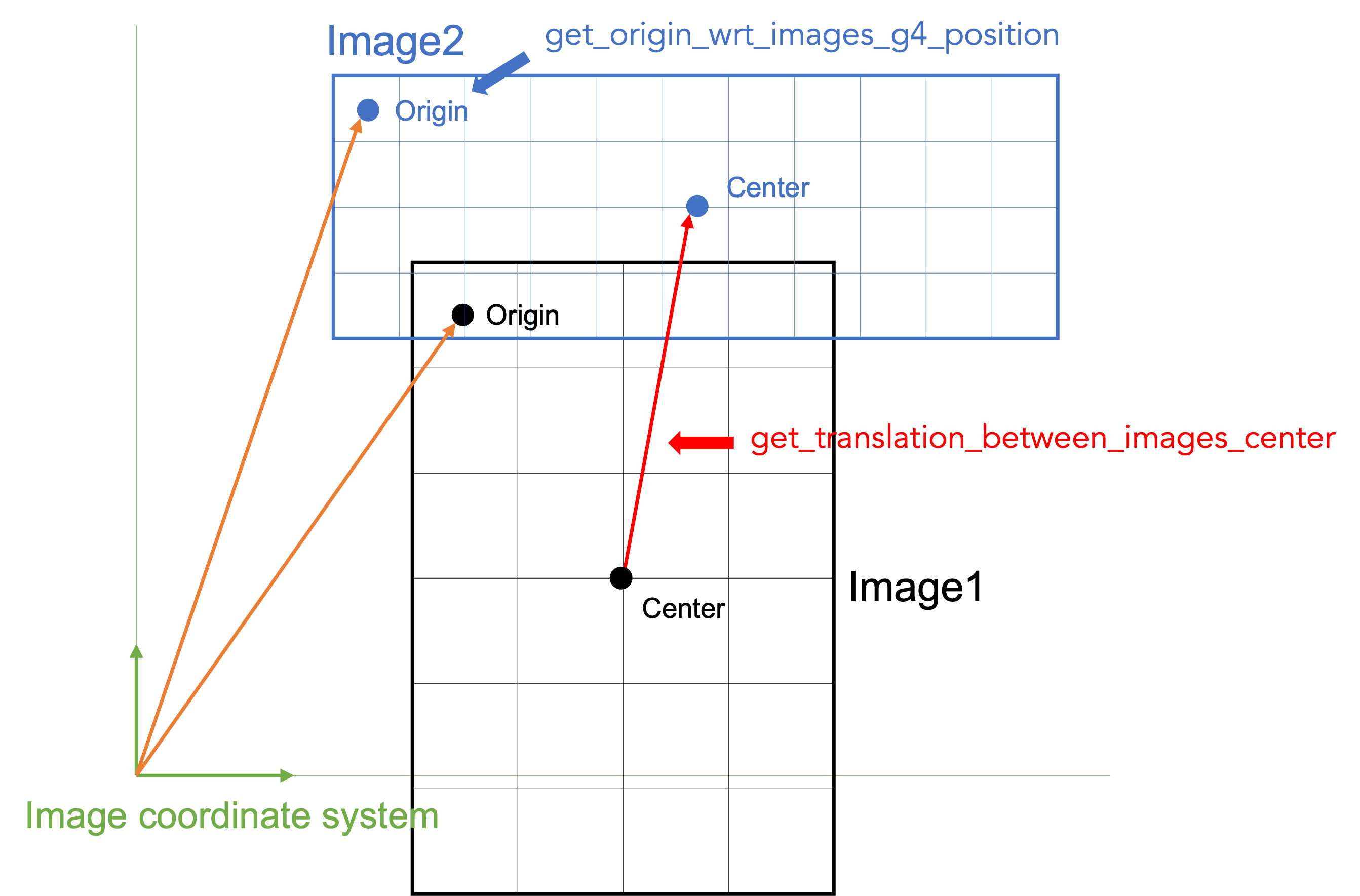
The DoseActor computes a 3D edep/dose map for deposited energy/absorbed dose in a given volume. The dose map is a 3D matrix parameterized with: dimension (number of voxels), spacing (voxel size), translation (according to the coordinate system of the “attachedTo” volume). There is possibility to rotate this 3D matrix for the moment. By default, the matrix is centered according to the volume center.
Like any image, the output dose map will have an origin. By default, it will consider the coordinate system of the volume it is attached to so at the center of the image volume. The user can manually change the output origin, using the option output_origin of the DoseActor. Alternatively, if the option img_coord_system is set to True the final output origin will be automatically computed from the image the DoseActor is attached to. This option call the function get_origin_wrt_images_g4_position to compute the origin. See the figure for details.
Several tests depict usage of DoseActor: test008, test009, test021, test035, etc.
1.2.6.3. PhaseSpaceActor
todo
1.2.6.4. Hits related actors (digitizer)
In legacy Gate, the digitizer module is a set of tool used to simulate the behaviour of the scanner detectors and signal processing chain. The tools consider list of interactions occurring in the detector (e.g. in the crystal), named as “hits collections”. Then, this collection of hits is processed and filtered by different modules to end up by a final digital value. To start a digitizer chain, we must start defining a HitsCollectionActor, explained in the next section.
1.2.6.4.1. DigitizerHitsCollectionActor
The DigitizerHitsCollectionActor is an actor that collect hits occurring in a given volume (or one of its daughters). Every time a step occurs in the volume a list of attributes is recorded. The list of attributes is defined by the user as follows:
hc = sim.add_actor('DigitizerHitsCollectionActor', 'Hits')
hc.mother = ['crystal1', 'crystal2']
hc.output = 'test_hits.root'
hc.attributes = ['TotalEnergyDeposit', 'KineticEnergy', 'PostPosition',
                 'CreatorProcess', 'GlobalTime', 'VolumeName', 'RunID', 'ThreadID', 'TrackID']
In this example, the actor is attached (mother option) to several volumes (crystal1 and crystal2 ) but most of the time, one single volume is sufficient. This volume is important: every time an interaction (a step) is occurring in this volume, a hit will be created. The list of attributes is defined with the given array of attributes names. The names of the attributes are as close as possible to the Geant4 terminology. They can be of few types: 3 (ThreeVector), D (double), S (string), I (int), U (unique volume ID, see DigitizerAdderActor section). The list of available attributes is defined in the file core/opengate_core/opengate_lib/GateDigiAttributeList.cpp and can be printed with:
import opengate_core as gate_core
am = gate_core.GateDigiAttributeManager.GetInstance()
print(am.GetAvailableDigiAttributeNames())
    Direction 3
    EventDirection 3
    EventID I
    EventKineticEnergy D
    EventPosition 3
    GlobalTime D
    HitUniqueVolumeID U
    KineticEnergy D
    LocalTime D
    ParticleName S
    Position 3
    PostDirection 3
    PostKineticEnergy D
    PostPosition 3
    PostStepUniqueVolumeID U
    PostStepVolumeCopyNo I
    PreDirection 3
    PreDirectionLocal 3
    PreKineticEnergy D
    PrePosition 3
    PreStepUniqueVolumeID U
    PreStepVolumeCopyNo I
    ProcessDefinedStep S
    RunID I
    ThreadID I
    TimeFromBeginOfEvent D
    TotalEnergyDeposit D
    TrackCreatorProcess S
    TrackID I
    TrackProperTime D
    TrackVertexKineticEnergy D
    TrackVertexMomentumDirection 3
    TrackVertexPosition 3
    TrackVolumeCopyNo I
    TrackVolumeInstanceID I
    TrackVolumeName S
    Weight D
Warning : KineticEnergy, Position and Direction are available for PreStep and for PostStep, and there is a “default” version corresponding to the legacy Gate.
Pre version |
Post version |
default version |
|---|---|---|
PreKineticEnergy |
PostKineticEnergy |
KineticEnergy (Pre) |
PrePosition |
PostPosition |
Position (Post) |
PreDirection |
PostDirection |
Direction (Post) |
At the end of the simulation, the list of hits can be written as a root file and/or used by subsequent digitizer modules (see next sections). The Root output is optional, if the output name is None nothing will be written. Note that, like in Gate, every hit such with zero deposited energy is ignored. If you need them, you should probably use a PhaseSpaceActor. Several tests using DigitizerHitsCollectionActor are proposed: test025, test028, test035, etc.
The two basics actors used to convert some hits to one digi are “DigitizerHitsAdderActor” and “DigitizerReadoutActor” described in the next sections and illustrated in the figure:
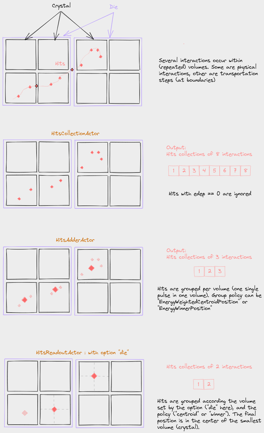
1.2.6.4.2. DigitizerHitsAdderActor
This actor groups the hits per different volumes according to the option group_volume (by default, this is the deeper volume that contains the hit). All hits (in the same event) occurring in the same volume are gathered into one single digi according to one of the two available policies:
EnergyWeightedCentroidPosition:
the final energy (“TotalEnergyDeposit”) is the sum of all deposited energy
the position (“PostPosition”) is the energy-weighted centroid position
the time (“GlobalTime”) is the one of the earliest hit
EnergyWinnerPosition
the final energy (“TotalEnergyDeposit”) is the one of the hit with the largest deposited energy
the position (“PostPosition”) is the position of the hit with the largest deposited energy
the time (“GlobalTime”) is the one of the earliest hit
sc = sim.add_actor("DigitizerAdderActor", "Singles")
sc.output = 'test_hits.root'
sc.input_digi_collection = "Hits"
sc.policy = "EnergyWeightedCentroidPosition"
# sc.policy = "EnergyWinnerPosition"
sc.group_volume = crystal.name
Note that this actor is only triggered at the end of event, so the mother volume to which it is attached has no effect. Examples are available in test 037.
1.2.6.4.3. DigitizerReadoutActor
This actor is the same as the previous one (DigitizerHitsAdderActor) with one additional option: the resulting positions of the digi are set in the center of the defined volumes (discretized). We keep two different actors (Adder and Readout) to be close to the previous legacy GATE versions. The additional option discretize_volume indicates the volume name in which the discrete position will be taken.
sc = sim.add_actor("HitsReadoutActor", "Singles")
sc.input_digi_collection = "Hits"
sc.group_volume = stack.name
sc.discretize_volume = crystal.name
sc.policy = "EnergyWeightedCentroidPosition"
Examples are available in test 037.
1.2.6.4.4. DigitizerGaussianBlurringActor
Digitizer module for blurring an attribute such as the time or the energy (single value only, not a vector). The blurring method can be “Gaussian”, “InverseSquare” or “Linear” :
For Gaussian: the sigma or the FWHM should be given blur_sigma or .blur_fwhm options.
For InverseSquare: blur_reference_value and blur_reference_value EQUATION
For Linear: blur_reference_value, blur_reference_value and blur_slope EQUATION
bc = sim.add_actor("DigitizerBlurringActor", "Singles_with_blur")
bc.output = "output.root"
bc.input_digi_collection = "Singles_readout"
bc.blur_attribute = "GlobalTime"
bc.blur_method = "Gaussian"
bc.blur_fwhm = 100 * ns
1.2.6.4.5. DigitizerSpatialBlurringActor
1.2.6.4.6. DigitizerEnergyWindowsActor
for spect
1.2.6.4.7. DigitizerProjectionActor
for spect
1.2.6.5. MotionVolumeActor
todo
1.2.7. Additional functionalities
The command line tool opengate_user_info allo to print all default and possible parameters for Volumes, Sources, Physics and Actors elements. This is very verbose but allow to have a dynamic documentation of everything currently available in the installed gate version.
The “contrib” folder contains additional functions that are useful but do not belong to the core of GATE.
The functions are used in several tests.
A readme file can be found : https://github.com/OpenGATE/opengate/tree/master/opengate/contrib/readme.md